Invitation to Modular Forms: Representation of an integer into sum of eight squares
Created: August 23, 2025 8:54 PM
Last Updated: September 13, 2025
Note: This is an edited reupload which is intended to be hosted on my blog. The reason is that I've received a performance issue complain from the old site hosted at Notion, so here is a spare one. There are minor typographical fixes but no new content changes.
Introduction
We’re interested in the following computational problem: Given n∈N, how many ways (i.e. number of tuples (x1,…,x8)∈Z8) are there such that n can be written as n=x12+⋯+x82.
Our basic computer programming knowledge tells us that we can design a naive algorithm as follows:
n = int(input())
ans = 0
for x1 in range(-n, n+1):
    for x2 in range(-n, n+1):
        for x3 in range(-n, n+1):
            for x4 in range(-n, n+1):
                for x5 in range(-n, n+1):
                    for x6 in range(-n, n+1):
                        for x7 in range(-n, n+1):
                            for x8 in range(-n, n+1):
                                if x1**2 + x2**2 + x3**2 + x4**2 + x5**2 + x6**2 + x7**2 + x8**2 == n:
                                    ans += 1
print(ans)
Of course, this takes a time complexity of O(n8), which is not very good. A basic obvious improvement is to observe that x2≥0 for all x∈N, so in order for a tuple to work, no entry can be larger than n because otherwise (say, if x1>n) we would have x12+⋯+x82>n+x22+⋯+x82≥n+1. This allows us to decrease the loop to the size of O(n).
n = int(input())
ans = 0
k = int(n**0.5)+1
for x1 in range(-k, k+1):
    for x2 in range(-k, k+1):
        for x3 in range(-k, k+1):
            for x4 in range(-k, k+1):
                for x5 in range(-k, k+1):
                    for x6 in range(-k, k+1):
                        for x7 in range(-k, k+1):
                            for x8 in range(-k, k+1):
                                if x1**2 + x2**2 + x3**2 + x4**2 + x5**2 + x6**2 + x7**2 + x8**2 == n:
                                    ans += 1
print(ans)
This takes time O(n4), a bit better, huh?
Obviously, from the eye of an algorithmist, we can do better. One direct way when we see something in this form is to do the meet-in-the-middle trick: instead of trying to solve for x12+⋯+x82=n, we solve for x12+x22+x32+x42=m and x52+x62+x72+x82=n−m, count the number of solutions to this, and sum over the scenarios for each m∈{0,…,n}. Let us try to implement.
n = int(input())

def count_sol(m):
    k = int(m**0.5)+1
    local_ans = 0
    for a in range(-k, k+1):
        for b in range(-k, k+1):
            for c in range(-k, k+1):
                for d in range(-k, k+1):
                    if a**2 + b**2 + c**2 + d**2 == m:
                        local_ans += 1
    return local_ans

ans = 0
for m in range(n+1):
    ans += count_sol(m) * count_sol(n-m)
print(ans)
The count_sol subroutine runs in time O(m4)=O(m2). We repeat the process 2(n+1) times, each of m≤n so the total time is in 2(n+1)⋅O(n2)=O(n3).
Can we do better? Still yes. Skilled algorithmists might even come up of this formulation immediately (note: I’m not that good though — I asked this problem to a bunch of friends and they immediately gave me the following formulation). We formulate this in terms of knapsack problem. Define dpi,j to be the quantity #{(x1,…,xi)∈Zi:∑k=1ixk2=j}, and look at what we can do about its recurrence.
In order to know the quantity dpi,j, we can enumerate all possible xi’s and observe that
Observe that the union in disjoint, so the cardinality of the whole is the sum of the cardinality of each case, so
dpi,j=1≤a≤j∑2dpi−1,j−a2+dpi−1,j.
With this formula, we can implement our dynamic programming algorithm as follows.
n = int(input())
dp = [[0 for j in range(n+1)] for i in range(9)]
dp[0][0] = 1
for i in range(1, 9):
    for j in range(0, n+1):
        dp[i][j] += dp[i-1][j]
        for a in range(1, int(j**0.5)+1):
            if j >= a**2:
                dp[i][j] += 2*dp[i-1][j-a**2]
print(dp[8][n])
This takes time O(n3/2), which is already very much improved from before. Is this the end? Can we do better? An algorithmist might give up at this point, but I refuse to give up just yet! Can we use some mathematical magic to improve this even more? It turns out that we can!
In this article, I’m going to invite you to the fascinating (quite relatively deep) theory of modular forms, not as just an algorithmist, but more as an algorithmic number theorist.
The prerequisites may be quite demanding in order to fill in all the gaps, but I intend to make this suitable to most general audiences, so for deep results from mathematics, if you’re not used to it, please feel free to “just assume the claim is true, move on to see how things fit, and try to understand the proof later”. The true prerequisites are:
Design and analysis of algorithms (and the fact that factoring an integer n is currently still not known to be doable in polynomial time in logn)
Introductory, real, complex, and Fourier analysis (basic ordinary differential equation, standard topology in R and C, differentiability, Lebesgue integration, dominated convergence theorem, Fourier transform, holomorphic function, contour integral, Laurent expansion)
Linear algebra (vector space, basis, dimension) and abstract algebra (group, group action, field)
Acknowledgement
I’d like to dedicate this section to thank my professor, Emmanuel Kowalski, for teaching me the basics of number theory and modular forms. I want to also thank a friend of mine, Pitchayut (Mark) Saengrungkongka, for helping me through mathematical obstacles during my studies. Finally, after all the messes I’ve made in my life, I’d like to thank everyone who still believes in me, who still believes that I can become a mathematician too, despite my sluggish brain and the distractions that slowed me down.
Disclaimer. Any mistakes found in this article belong to me. I’m more than happy to receive feedback and report of errors.
Now let us begin.
Modular Forms
Note. The main reference for this whole section is the course Number Theory II: Introduction to Modular Forms given by Emmanuel Kowalski (see https://metaphor.ethz.ch/x/2025/fs/401-3112-23L/). Other small references will be given throughout the article.
It is quite surprising that modular form is a structure that is studied extensively and, even though initially it is of number theoretic nature, it now has applications in very different areas of mathematics. When I first see it, it looks very artificial, as if it comes out of nowhere. (Who on earth would have think up of this structure???) The following quote is taken from Martin Eichler.
There are five fundamental operations in mathematics: addition, subtraction, multiplication, division and modular forms.
So what is a modular form? In simple terms, it is a function f:H→C that satisfies the following property (here H:={z∈C:Im(z)>0} is the Poincaré upper-half plane):
There exists an integer k≥0 such that f(cz+daz+b)=(cz+d)kf(z) for all z∈H and for all a,b,c,d∈Z such that ad−bc=1.
If furthermore, f is holomorphic everywhere in H, we say that it is a holomorphic modular form of weight k and of level 1. For meromorphic modular forms, we don’t require f to be defined on the whole H — there can be isolated poles, only that the relation f(cz+daz+b)=(cz+d)kf(z) holds for all z such that f(z) is defined (i.e. not a pole). We will generalize to other levels later.
Now we ramp up the machinery a bit for some spiciness. Define GLn(K) as the set of n×n invertible matrices with entry in the field K. Equivalently, it is the set of n×n matrices with nonzero determinant. Since det(AB)=det(A)det(B) for square matrices A,B of the same size, and by invertibility, we see clearly that GLn(K) has a group structure defined by multiplication. Now, we define a subset SLn(K)⊆GLn(K) as the subset of matrices with determinant one. This subset is also a group, so it’s a subgroup. We can generalize this a bit for the case that K is not a field, for GLn(K) it looks like we run into an immediate problem: it’s not a group anymore. However, fortunately, for SL2(Z), there is no problem. If (acbd)∈SL2(Z) is a matrix with determinant one, i.e. ad−bc=1, then consider the matrix (−dcb−a). We have
This means (−dcb−a) is the inverse of (acbd)! So SL2(Z) forms a group.
Now, define a group action ∣k of SL2(Z) acting from the right on the space of functions H→C by
fk(acbd):=(z↦f(cz+daz+b)(cz+d)−k).
It restricts to the space of holomorphic functions. Now, in fancier words, we can define modular forms of weight k and of level 1 to be functions f:H→C such that f∣kg=f for all g∈SL2(Z), i.e., it is the subset of (SL2(Z),∣k)-invariant functions. In particular, it is enough to show that f is invariant under a generating set of SL2(Z) to conclude that it is invariant under the whole group. We will use this fact later.
Definition. (Modular form of weight k and of level 1) A function f:H→C is said to be a modular form of weight k and of level 1 if f is invariant under the group action ∣k of the group SL2(Z).
Now, consider the action of SL2(Z) on H defined by (acbd)⋅z=cz+daz+b. This action sends point of H to another (or maybe the same) point of H. We can start by just being randomly curious about this and ask interesting questions on this action. First of all, given a fixed z∈H, what is the orbit of this point by the action? Well, we can pick (1011) from SL2(Z) and observe that it sends z to 0z+11z+1=z+1. Therefore, z+n is inside the orbit, for all n∈Z. Of course, this is not the end. Let’s try something different. Try (01−10)∈SL2(Z). This sends z↦z−1. It may be hard to visualize at first, but observe that if ∣z∣>1, it sends to ∣z−1∣=∣z∣1<1. This means, a point outside the unit disk can be sent into somewhere inside the unit disk. This allows us to conclude that “it is enough to just consider points inside a strip [z0,z0+1] because the points outside this strip can be reached from one inside this strip by applying the group action” and also “it is enough to just consider points inside the unit disk because points outside the unit disk can be reached by the z↦−1/z transformation”. Turns out this is something that we’ll state it in more precise terms and use it repeatedly afterwards (but for reasons that will come later, instead of inside the disk, we’d rather use outside the disk).
The Fundamental Domain
Definition. The fundamental domain is defined as D:={z∈H:∣z∣≥1;∣Re(z)∣≤21}.
Theorem 1 [Serre, Ch. VII, §1, Th 1. and 2.].
For every z∈H there exists g∈SL2(Z) such that gz∈D.
Suppose z,z′∈D are two distinct points, such that there exists g∈SL2(Z) with z′=g⋅z, then either (a) Re(z)∈{−21,21} and z=z′±1, or (b) ∣z∣=1 and z′=z−1.
For all z∈D∘, StabSL2(Z)(z)={id}.
The group SL2(Z) is generated by S=(01−10) and T=(1011).
Proof. Define G′:=⟨S,T⟩≤SL2(Z). We will eventually show that G′=SL2(Z) later, but now let us show 1. Take z∈H, and let g=(acbd)∈G′be arbitrary first (we will fix it later). We have
(We used the simple facts that a,b,c,d∈Z, so c=c;d=d. We know that ad−bc=1, and we know that Im(z)=−Im(z).) Now, the idea is that for a given z, we will try to send it as far away (from the origin) as possible, then slide back by repeatedly applying T until it stays in D. For any fixed M>0, The set Sz,M:={(c,d)∈Z2:∣cz+d∣≤M} is finite. To see this, write z=x+iy and observe that ∣cz+d∣≤M if and only if M2≥∣cz+d∣2=∣c(x+iy)+d∣2=(cx+d)2+(cy)2. So if (c,d) is in that set, then ∣c∣≤∣y∣M (finitely many choices), and for a fixed c, the integer d must satisfy ∣cx+d∣≤M, that is, d∈[−cx−M,−cx+M], which contains finitely many integers. This proves that the set Sz,M is finite. If we fix M=∣z∣, then we see that (1,0)∈Sz,M, so the set is not empty. Furthermore, we’re looking for such pair with smallest ∣cz+d∣, so enlarging M wouldn’t help. This means min(c,d)∈Z2∣cz+d∣ exists, with (c,d)∈Sz,∣z∣. However, we want to only look at pairs corresponding to elements of G′, so we consider the set
S~z:={(acbd)∈G′:∣cz+d∣≤∣z∣}.
Well, S∈S~z so it is not empty, and there are only finitely many choices of (c,d) here, so, to minimize ∣cz+d∣, we loop over all possible pairs in Sz,∣z∣, and check if there exists a pair (a,b) making (acbd)∈S~z. We don’t need to loop over all possible (a,b). Just that if one exists, we track the minimum over such ∣cz+d∣. This shows that there exists g∈S~z minimizing ∣cz+d∣.
Now that we got g∈G′, we want to slide gz back into the strip [−21,21]+iR>0. Indeed, pick n∈Z such that n+gz∈[−21,21], and so Tngz∈[−21,21]. Furthermore, we have ∣Tngz∣≥1 because otherwise ∣Tngz∣<1 and so when we consider STng∈G′ we get
Im(STngz)=∣Tngz∣Im(Tngz)>Im(Tngz)=Im(gz),
a contradiction of the maximality of Im(gz) for g∈G′. This shows that Tngz∈D.
Phew. That was long. Now let us move to the second point (which is even longer, because I want to make it very clear to myself, and not leave the casework to the reader). We want to now show that if two points inside the fundamental domain are congruent modulo G′, then they must be in a few special cases only. Suppose z,z′∈D are two distinct points and (acbd)=g∈G′ such that z′=gz. Assume without loss of generality that Im(z)≤Im(z′) (otherwise just swap z and z′). And so Im(z)≤Im(gz)=∣cz+d∣2Im(z), so ∣cz+d∣≤1. Write now z=x+iy with ∣x∣≤21 and y>23. If ∣c∣≥2 , then
a contradiction. So ∣c∣<2, i.e. c∈{−1,0,1}. If c=0 then ∣cz+d∣≤1 implies d∈{−1,1} (remember that c=d=0 is not possible since this means detg=0, impossible in G′⊆SL2(Z)). Furthermore, in SL2(Z), we have ad−bc=1 so for c=0, ad=1 means a=d. This means z′=gz=daz+b=z±(integer), but z,z′∈D so such integer must be ±1 only. And in this case, ∣Re(z)−Re(z′)∣=1, so they must lie on somewhere inside the vertical boundaries of D. This concludes that in case c=0, we have Re(z)=±21 and z′=z±1, i.e., case (a) in the theorem.
Now, for the case that c∈{−1,1}, we have 1≥∣cz+d∣=∣cx+icy+d∣=(cx+d)2+y2≥(cx+d)2+(23)2=(cx+d)2+43. This means ∣cx+d∣≤21. This means d cannot be too far away, say, ∣d∣>1 is not possible, because then cx∈[−d−21,−d+21] is impossible for ∣cx∣=∣x∣≤21. For d=−1, the only possible place for cx to be is 21, and in this case, 1≥∣cz+d∣2=(cx+d)2+y2=41+y2, so 23≤y≤23, i.e., y=23, and for d=1, cx=−21, and 1≥∣cz+d∣2=41+y2 so y=23 as well. In these two subcases, we have z=±21+i23, and so ∣z∣=1.
In both subcases, we have d+2cx=0. Consider the fact that gz=z′∈D, so ∣Re(gz)∣≤21, i.e. that
But we knew that ∣cz+d∣≤1, so 21≥∣acx2+bcx+adx+bd+acy2∣. In both subcases, 1=∣z∣2=x2+y2, so we have 21≥∣ac+(bc+ad)x+bd∣=∣ac+(2bc+1)x+bd∣=∣b(d+2cx)+ac+x∣=∣ac+x∣. If ∣a∣≥2, then 2≤∣ac+x−x∣≤∣ac+x∣+∣x∣=∣ac+x∣+21, a contradiction, so a∈{−1,0,1}.
Observe that in both subcases, 2cxd=−1. If b=0, then ad=1+bc means ad−1 also cannot be zero, i.e. ad=1. If a=−d then 21≥∣ac+x∣=∣−dc+x∣=∣x−cdx+x2∣=∣±2121+41∣=23, a contradiction, so the only option when b=0 is that a=0. In such scenario, 1=ad−bc=−bc so b=−c. Now for b=0, we have 1=ad−bc=ad so a=d.
To summarize, for the case (b.1) that c∈{−1,1} and d=0, we have deduced the candidates for g:
g∈{(0c−cd):cx=−2d}∪{(dc0d):cx=−2d}.
If g is in the first set, gz=cz+d−c=c(x+iy)+d−c=2d+ic23−c=2cd+i23−1=−x+iy−1=x−iy1=z1=∣z∣2z=z, a contradiction with the fact that z′=z. If g is in the second set, gz=cz+ddz=cz+ddzcz+dcz+d=∣cz+d∣2(dz)(cz+d)=dc∣z∣2+d2z=cd+z=−2x+x+iy=−x+iy=−zˉ=−zzzˉ=−z1, and now it is clear that g=(1−2x01) or g=(−12x0−1) for the case (b.1).
Now we’re left with the case that c∈{−1,1} and d=0 (b.2). In this case, 1=ad−bc=−bc so b=−c. We’ve assumed that 1≥∣cz+d∣, but for d=0 and ∣c∣=1, this means ∣z∣=1. Recall that ∣Re(gz)∣≤21 implies that 21≥∣acx2+bcx+adx+bd+acy2∣. Plug in what we have to get 21≥∣acx2−c2x+acy2∣=∣ac(x2+y2)−x∣. Suppose ∣a∣≥2, then, we have, by triangle inequality, that ∣ac(x2+y2)∣≤∣ac(x2+y2)−x∣+∣x∣, and so
a contradiction. So, a∈{−1,0,1}. If a=0, then a=±1, so ac=±1, and 21≥∣Re(gz)∣=∣cz+d∣21∣(ax+b)(cx+d)+acy2∣=∣(ax−c)(cx)+acy2∣=∣acx2+acy2−x∣=∣ac∣z∣2−x∣=∣ac−x∣ would mean x must be near ac=±1 with distance no more than 21. The only case is back to when ∣x∣=21, and this shows that y=23 and ∣Re(gz)∣=21 also in this case. Furthermore, if ac=−1 then x=−21 and if ac=1 then x=21. We can summarize this as 2acx=1 (or equivalently ac=2x). This shows that ∣gz∣2=∣cz∣2∣az−c∣2=(ax−c)2+(ay)2=2−2acx=1, so ∣gz∣=1 also. Now, we have
a contradiction. This rules out a=±1. Now let us check a=0. We have
gz=cz−c=z−1.
This shows that for c=0, ∣z∣=1 and z′=−z1, and completes the case (b).
Now the third part follows by the same argument as in the previous part: Take z∈D∘. Suppose g=(acbd)∈StabSL2(Z)(z), then gz=z. We have Im(gz)=∣cz+d∣2Im(z)=Im(z), so ∣cz+d∣=1. By the same argument as before, it is impossible for ∣c∣≥2, so we know that c∈{−1,0,1}. If c=0 then we follow the same argument as before to deduce that z=±21+23i, a contradiction since we’ve assumed that z is in the interior, so we conclude that c=0;d=1, and ad−bc=1 implies a=1. This means z=gz=cz+daz+b=z+b, so b=0 and this tells us that StabSL2(Z)(z)⊆{id}.
Now let us show the fourth part, that G′=SL2(Z). Take g∈SL2(Z) and let us show that g∈G′. Choose z0:=2i∈D∘, and let z=gz0∈H. We’ve seen that by 1., there exists g′∈G′ such that g′z∈D. The points z0 and g′z=g′gz0 are both in D and are congruent modulo G′. But z0 is not on the boundary, so both points fail to be distinct. Therefore, g′gz0=z0∈D∘. So g′g∈StabSL2(Z)(z0)={id}, i.e. g=g′−1∈G′. This shows that SL2(Z)⊆G′ and hence completes the proof. □
We now turn to the more restricted notion: holomorphic modular forms which is also defined and holomorphic at infinity.
At Infinity
The real line R is not compact. The sequence 1,2,3,… has no accumulation point in R. However, we can compactify it by adding a point at infinity, say, define R^:=R∪{∞}. In the same way, the complex plane is not compact, but we can think of it as a sphere with one punctured hole corresponding to ∞.
Now, with this picture in mind, we go back to modular forms and try to complete them at infinity.
Proposition 2. Let f be a meromorphic modular form of weight k, then there exists a meromorphic function f~:D×∖{isolated poles}→C such that f(z)=f~(e2πiz) for all z∈H∖{isolated poles}, where D×:={z∈C:0<∣z∣<1}.
Proof. First, for any a∈R, there is a bijection
Φa:{Stripaz→D×∖{re2πia:0<r<1}↦e2πiz
where Stripa:={z∈C:Re(z)∈(a,a+1);Im(z)∈(0,+∞)}, which is very nice in our use case. Furthermore, Φ is holomorphic everywhere in its strip, and we can compute the derivative as Φ′(z)=2πie2πiz which never vanishes in the strip. This shows that Φ is a conformal equivalence. Now, we can define f~ by patching up two charts. The first chart is Φ−21sending our favorite strip to D×∖(−1,0), and the second chart is Φ21 sending an offset strip to D×∖(0,1). We define f~(q) as f(Φ−21−1(q)) whenever q∈D×∖(−1,0) and define as f(Φ0−1(q)) whenever q∈D×∖(0,1). Observe that this is well-defined (except for some not too many points that are not defined even on f since it’s meromorphic) since the values agree on the intersection. Indeed, if q∈D×∖(−1,1) then z−21:=Φ−21−1(q) and z0:=Φ0−1(q) satisfies e2πiz−1/2=e2πiz0, so e2πi(z−1/2−z0)=1. This means n:=z−1/2−z0∈Z, and so f(z−1/2)=f(z0+n)=f((10n1)z0)=(0z0+1)kf(z0)=f(z0) by the modularity of f (if it is defined there). The two charts extend each other to f~:D×→C, which is meromorphically defined, such that f(z)=f~(e2πiz) for all z∈H wherever defined. (One can check this by sliding z back to our favorite strip or the offset strip, and note that f is periodic due to modularity, and z↦e2πiz is already periodic by default) □
Note. Inspecting the proof carefully, we haven’t actually used the (rather strong) fact that f is modular. We’ve only used the fact that f is periodic. We will recall this construction for “just periodic, but not necessarily modular” meromorphic functions later on.
So now the disk D× is our model for H. Think of it as the upper hemisphere of the Riemann sphere, with the center removed. Do you see the point of doing this now? If we can complete f~ at the hole, we would complete f at infinity! If there is a meromorphic continuation of f~ to all of D:=D×∪{0}, then we’re done.
Definition. A meromorphic modular form f is said to be meromorphic at infinity if there exists a meromorphic continuation of f~ to D. It is holomorphic at infinity if f~ is holomorphic at 0. If f~ is defined at 0, we may write f(∞) to denote f~(0).
Fourier Expansion
For meromorphic modular form that is also meromorphic at infinity, by complex analysis, we can expand f~ into a Laurent series f~(q)=∑n≥kanqn for some k∈Z (maybe negative) and for some sequence (an)n≥k of complex numbers with ak=0, such that equality holds for all q in a neighborhood of 0 (except maybe zero itself if k<0). Such expansion is unique, i.e., for a given f, the pair (k,(an)n≥k) is uniquely defined (even if we pick different neighborhoods, the pair coincides). Equivalently, we have f(z)=∑n≥kane2πinz for all z with large enough Im(z), with an extra value of f(∞)=∑n≥kan. To simplify things, we would rather denote (an)n∈Z but keep in mind that it is always zero when the index is negative enough.
Definition. For a meromorphic modular form f that is also meromorphic at infinity, there exists a unique sequence (an)n∈Z of complex numbers, which takes value zero when the index is negative enough, such that f~(q)=∑n∈Zanqn in a neighborhood of zero but maybe without zero itself. The sequence is called the Fourier expansion of f at infinity, and the sequence is called the Fourier coefficients.
Definition. We write Mk for the set of holomorphic modular forms of weight k, which is also holomorphic at infinity, and we write Sk for the subset of those forms that take value 0 at infinity.
Also observe that the Fourier coefficients starts at n≥0 for forms in Mk and starts at n≥1 for forms in Sk.
Now that we’ve defined Mk and Sk, what do you see? This is where things get interesting.
Proposition 3. For f,h∈Mk and λ∈C, we have f+h∈Mk and λf∈Mk. The result is still true if we replace Mk by Sk.
This checks that the modularity condition still holds. The fact that they are holomorphic and also holomorphic at infinity is a standard fact from complex analysis. Same thing holds when we replace Mk by Sk. Easy to check that they still attain zero at infinity. □
This shows that Mk is a vector space, and Sk is a subspace.
Soon, we will want to study the shape of Mk and Sk. Let us just be curious about these objects, and so we can ask natural questions: Can we compute the dimension of the spaces for each weight? Is there an explicit formula? Furthermore, can we find a basis for them? It turns out that luckily, we can do all of that. But anyway, we need some heavy complex analytic machinery here first.
The Valence Formula
Here I’m going to follow almost exactly the same as in [Serre, Ch. VII, §3, 3.1.], but written in my own wording (and I’ll try to simplify as much as I can).
From complex analysis, for any meromorphic function f≡0 in an open set U, if we fix a∈U then we can find a neighborhood N of a inside U and a Laurent expansion ∑n≥kan(z−a)n (with ak=0) such that the expansion coincides with f in N∖{a}. Such expansion is unique, even if the neighborhood is not, that is, even in a different choice of neighborhood, the expansion is still the same. The number k is called the order of vanishing of f at a, and is denoted by orda(f). The residue of f at a, denoted by Resz=a(f(z)) or Resa(f), is defined as a−1.
Let us first set up the complex-analytic machinery.
Lemma 4. For a meromorphic function f defined on an open set U, and for a point a∈U, we have
Resa(ff′)=orda(f).
Proof. Write the Laurent expansion of f at a as ∑n≥kan(z−a)n, ak=0. Put g=∑n≥k+1an(z−a)n, then, in a neighborhood of a except at a, we have
which, after plugging in z=a, gives ak−kak+1, i.e., well-defined without a pole, so the function z↦ak(z−a)k+gg′−gk(z−a)−1 is holomorphic in that neighborhood, i.e. its Laurent series is Taylor, and so the residue of f′/f must be k, which is the order of f at a. □
Recall the basic formula from complex analysis (Cauchy Integral Formula): If f:U→C is a holomorphic function on an open set U, let γ:S1→U be a null-homotopic Jordan curve with Jordan interior N such that N⊆U and with winding number +1. Then, for any a∈N, we have
2πi1∫γz−af(z)dz=f(a).
Lemma 5. Suppose U⊆C is an open set, where f:U→C is holomorphic. We define, for any a∈U;r>0;α∈(0,2π];θ∈R such that the disk {a+z∈C:∣z∣≤r} is contained in U, the curve
γa,r,α,θ:{[0,1]t→C↦a+rei(θ+tα).
Then, we have for any a∈U
r→0r>0lim∫γa,r,α,θz−af(z)dz=iαf(a).
Proof. Since f is holomorphic at any a∈U, we fix a∈U then there exists a Taylor expansion in a neighborhood N of a in U. By definition of a neighborhood, there exists a closed disk of some radius R centered at a that lies entirely in N. Write f(z)=f(a)+g(z)(z−a) with g holomorphic. This equality holds in N. Now, we fix θ∈R, and we have, for 0<r≤R,
and consider the compact disk {a+z:∣z∣≤R}⊆N. Its image under z↦∣g(z)∣ must also be compact, so we can bound ∣g(a+rei(θ+tα))∣≤C for some constant C not depending on r. This means
Now we bring another tool from the basic complex analysis toolbox. (Cauchy’s Argument Principle). For a meromorphic function f meromorphic on an open set U⊆C, if γ:S1→C is a null-homotopic Jordan curve with winding number +1 and with Jordan interior N⊆U, then
∫γff′=2πiz∈N∑ordz(f).
Corollary 6. For a meromorphic function f meromorphic on an open set U⊆C, for any a∈U, reusing the notation of curves from Lemma 5., we have
r→0r>0lim∫γa,r,α,θff′=iαorda(f).
Proof. Recall from Lemma 4. that in some neighborhood N of a∈U, we have that f′/f≡z−aorda(f)+g is the Laurent expansion at a, with g holomorphic. Apply Lemma 5 on z↦orda(f)+g(z)(z−a), which is holomorphic in a (maybe another) neighborhood N′ of a, to see that
Now observe that in N∩N′, the meromorphic equality ff′≡z−aorda(f)+g is actually defined, i.e., that f(z)f′(z)=z−aorda(f)+g(z) for all z∈N∩N′. This shows that
r→0r>0lim∫γa,r,α,θff′=iαorda(f)
and hence completes the proof. □
Now our complex analysis toolbox is complete, and we’re ready to proceed to our case of meromorphic modular forms of weight k. Define ord∞(f) to be ord0(f~).
Theorem 7. Let f≡0 be a meromorphic modular form of weight k. One has
Proof. First, we observe that there are finitely many zeros and poles. Indeed, since f~ is meromorphic at zero, there exists a neighborhood (and hence we can assume to be a smaller disk) U={z∈C:0<∣z∣<r} such that f~ has neither zeros nor poles in U. This means f has neither zeros nor poles when 0<∣e2πiz∣<r. Writing z=x+iy, this is equivalent to 0<∣e2πi(x+iy)∣<r, but e2πi(x+iy)=e2πixe−2πy so this is equivalent to −2πy<logr, which is y>2π−logr=2πlog(1/r). So zeros and poles of f must have imaginary part no more than 2πlog(1/r). Now, the set Dr:=D∩{x+iy∈H:y≤2πlog(1/r)} is compact, and so there can be only finitely many zeros and poles.
Now we set up an integral over the contour Dr.
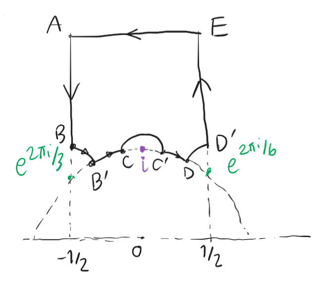
Let ΓR denote the boundary curve of Dr minus small disks of radius R around e2πi/6,i,e2πi/3, going counterclockwise, with any parametrization with nonzero speed. Suppose first that there is no zero and no pole of f on the boundary curve ΓR. We will take care of this later. We have, by the Cauchy’s argument principle, that
∫ΓRff′=2πiz∈Dr∑ordz(f).
Now, we try to do the same integral but from another point of view. First, the segment EA gets mapped by the conformal equivalence to a circle C in the unit disk. Let D be the disk such that its boundary is C. This means
Observe that f~(e2πiz)=f(z), so 2πif~′(e2πiz)=f′(z). The equality before the last comes from the fact that we’ve already assumed that there are no zeros or poles of f in the higher region of our favorite strip, and so this means there are no zeros or poles in D∘∖{0}.
since the fact that f(−1/z)=zkf(z) tells us that f′(−1/z)z−2=kzk−1f(z)+zkf′(z) and so f′(z)=f′(−1/z)z−k−2−kz−1f(z)=f′(−1/z)z−k−2−kz−k−1f(−1/z). Simplifying this, we have
Now we’re left with taking care of the removed disks. For BB′, we have
∫BB′ff′=−∫γ2πi/3,R,αR,θRff′
where αR is the arc angle of BB′, and θR is the offset angle. Observe that as R tends to zero, αR tends to 3π. The same argument applies for DD′. Same for CC′ but the angle tends to π instead.
Now we’re left with handling the case where there exists some zeros or poles on Γ0∖{e2iπ/3,e2iπ/6,i}. Note that we don’t have to worry in the process of taking R→0 because zeros and poles are isolated, and so the limit still works (we can just skip those R’s). In this limiting scenario, B and B′ coincide, same for (C,C′) and (D,D′). If z∈AB is a zero or a pole, then by modularity, z+1∈DE would also be the same. We can edit ΓR by perturbing it by a disk of a very small radius.
In this way, the integral would stay the same, but the sum of orders will count this point once. In order to avoid problems of double counting, we denote by ∑z∈Dr/SL2(Z)ordz(f) instead of simply summing over the whole contour (or just the interior). Now we’re left with dealing with zeros and poles on the arc BCD∖{i,e2πi/3,e2πi/6}. We apply the same trick, but when we see any problem point z now we will also see the congruent one at −1/z. We can just put two disks, remove one from the contour and indent one to the contour. This completes the proof. □
First Examples of Modular Forms: Eisenstein Series and Poincaré Series
When I was writing everything before this, I thought I could skip these explicit examples and then move on to our special case, but now I changed my mind and I think that it’s a nicer way to approach the subject by introducing these explicit examples.
The thing is, even if I said it’s “explicit”, it’s not that explicit. I’ll begin by showing the idea and then move on to the definition.
Let’s play a little game here. If I have a grid with n rows and m columns, in each cell there exists at most one object, and I have some function f that has its value depending on the multiset of objects in each row (not depending on order). What happens now? If we permute the columns of the grid, then the multiset of objects in each row doesn’t change, and so the value of this grid under f stays the same, right? Now if we want to construct a function that has its value preserved under permutations of rows and permutations of columns, how would we construct? We would define
f~(grid):=σ permuting rows∑f(σ⋅grid).
And now, for any permutation σ of rows, of columns, or composition of both, we have f~(σ⋅grid)=f~(grid).
Now I’ll take this to the algebraic setting and make it more precise.
Lemma 8. For a group G, a subgroup H of G, a set X in which G acts on X, and a function f:X→C which is H-invariant (i.e. f(hx)=f(x) for all h∈H and x∈X), we can define
f~(x):=gˉ∈H\G∑f(gx).
If the sum makes sense, i.e., if it converges absolutely, then f~(gx)=f~(x) for all g∈G and x∈X.
Proof. First, f~ is well-defined, because for two elements g1 and g2 in G corresponding to the same coset, we have Hg1=Hg2, i.e., there exists h∈H with h=g2g1−1. This means f(g2x)=f(g2g1−1g1x)=f(hg1x). But f is H-invariant, so this is actually f(g1x). This means one can take any element in the same coset inside the sum. The condition of absolute convergence implies that we can commute the sum however we want.
Now, pick any g′∈G. We have
f~(g′x)=gˉ∈H\G∑f(gg′x).
But Φ:Hg↦Hgg′ only permutes the cosets in H\G. Indeed, for any coset Hg0 we can pick g=g0g′−1 then Φ(Hg)=Hgg′=Hg0g−1g′=Hg0, so Φ is surjective. Now if Hg1g′=Hg2g′, then g2g′g′−1g1−1∈H means there exists h=g2g′g′−1g1−1 and so hg1=g2, i.e., Hg1=Hg2, so Φ is injective. This means the sum inside can be rewritten as the original form, and so f~(g′x)=f~(x). □
We will adapt this idea into our settings of modular forms. Let G:=SL2(Z), H:=⟨±T⟩, and X:=H. Then there exists a very simple function that is ±T-invariant (i.e. periodic). Fix m∈Z and define
fm(z):=e2πimz.
This is periodic. Now we can do something similar to the lemma above, but adapt things a bit to make it satisfy the modularity condition. Define
where g′′=gg′, with g′′=(a′′c′′b′′d′′). This Pm,k is called the Poincaré series, and for m=0 it is called the Eisenstein series, denoted by Ek:=P0,k. We’ve showed that if they are well-defined, then they are modular forms of weight k. We’re now left with showing that they are well-defined, i.e., that the series converges absolutely.
Proposition 9. For even k≥4 and m≥0, the series Pm,k converges locally uniformly absolutely for all z∈H.
We know that gz∈H for all g∈SL2(Z), so we may write gz=x+iy with y>0, and observe that e2πimgz=e2πim(x+iy)=e2πimx−2πmy, and so its absolute value (i.e. complex modulus) is e−2πmy, which is between zero and one. This means
Let us now show the convergence for ∑gˉ∈⟨T⟩\SL2(Z)∣cz+d∣−k. We claim that for each (c,d)∈Z2 with gcd(c,d)=1, there exists (a,b)∈Z2 such that (acbd)∈SL2(Z). Furthermore, if there are multiple candidates, then they belong to the same coset. To show this, fix (c,d)∈Z2 with gcd(c,d)=1. By Bézout’s identity from elementary number theory, there exists an integer solution (a0,b0)∈Z2 satisfying a0d−b0c=1. This is a linear Diophantine equation, and so all solutions are described by (at,bt), defined by at=a0+ct and bt=b0+dt for t∈Z. Now we’re left with showing that (a0cb0d) and (atcbtd) belong to the same coset for all t∈Z. Indeed, we have
This shows that they belong to the same coset. Now, also observe that elements from the same coset have the same (c,d). This means what we were doing is essentially defining a projection
π:⟨±T⟩\SL2(Z)→{(c,d)∈Z2:gcd(c,d)=1},
sending (acbd) to (c,d), and showed that it is well-defined, injective, and surjective, hence a bijection. Now we go back to the sum and see that
Now we recall some basic facts from analysis. In R2, all norms are equal. Observe that (x,y)↦∣xz+y∣ is a norm, so there exists α(z),β(z)>0 such that for all (x,y)∈R2, α(z)∣xz+y∣≤max(∣x∣,∣y∣)≤β(z)∣xz+y∣. This means
where the last inequality follows from counting integer lattice points (c,d) that has max(∣c∣,∣d∣)=r. (They are integer lattice points on the square of side length 2r+1. Remove one from each side to avoid double counting, then multiply by four to count them all.) Observe that for k>2, this converges, so in particular, for k≥4, the Poincaré series converges absolutely for fixed z. Now, let us show that it converges locally uniformly absolutely. We can actually define α(z)1:=sup(x,y)=(0,0)max(∣x∣,∣y∣)∣xz+y∣=supmax(∣x∣,∣y∣)=1∣xz+y∣. This is continuous, so for fixed z, one can pick a small compact neighborhood K of z and then the value of α(z′) for z′∈K will be bounded away from zero and infinity. This proves that the convergence is locally uniform. □
Now that Pm,k is locally uniformly absolutely convergent, for any m≥0 and k≥3, we observe that each piece z↦fm(z)(cz+d)−k is a holomorphic function, and so the sum over all pieces in a locally uniformly absolutely convergent series must also be holomorphic. This means the following.
Corollary 10. For any m≥1 and even k≥4, we have Pm,k∈Sk, and for m=0,P0,k=Ek∈Mk∖Sk.
Proof. We’ve shown the holomorphicity in H, and that they satisfy the modularity condition. Now we’re left with studying their behavior at infinity. We have, for m≥1, that
For the trivial coset, we have (c,d)=(0,1), and so the term inside is one. For the rest, the terms inside tends to zero, and so we have Ek(∞)=1, so Ek∈Mk∖Sk. □
It seems like we’ve constructed a huge family of modular forms, namely the Poincaré series. However, this is a bit far from obvious, but a lot of them turn out to be zero, so we get nothing new. Anyway, the Eisenstein series are surely not zero, since they extends to one at infinity.
The Space of Holomorphic Modular Forms
Now we’re ready to study Mk and Sk. Recall that Mk is the space of holomorphic modular forms that are also holomorphic at infinity. This means, if f∈Mk, then ordz(f)≥0 for all z∈H∪{∞}. Before we continue, observe that if f is a modular form, we have
The idea here is to try to solve the equation (solve for ordz(f)) given by the valence formula.
Let us begin with M0. For k=0, the right hand side is zero, and we knew that the orders of a holomorphic modular form that is also holomorphic at infinity must be nonnegative, so the only possible outcome is the the order of f is everywhere (including at infinity) is zero! This means ∣f∣ is bounded away from zero and infinity. Let f(z)=f~(e2πiz)=∑n≥0ane2πinz be its Fourier expansion at infinity. Recall the fundamental domain D:={z∈H:∣z∣≥1;∣Re(z)∣≤21}. We thicken the fundamental domain by a small margin ε>0 (to make it concrete one can just pick ε:=1001) and define Dε:={z∈H:dist(z,D)<ε}. We push Dε into the conformal equivalence Φ and send it into an open subset of the disk. This misses the point at infinity (zero of the disk), so we complete it and define Dε′ˉ:=Φ(Dε)∪{0}. This is very similar to an open disk (except maybe the boundary isn’t a perfectly round circle) inside the unit disk. We also send the original fundamental domain (with completion) to the unit disk as D′ˉ:=Φ(D)∪{0}. Now this is a compact disk inside the unit disk, and D′ˉ⊆Dε′ˉ. By the maximum modulus principle, if f~ is not constant, there cannot be a local maximum of f~ inside Dε′ˉ. But since f is modular, the image of f under H∪{∞} is already presented by the image of f under D∪{∞}, which is the image of f~ under D′ˉ, so a global maximum of f (including maybe at infinity) must correspond to a local maximum of f~ inside Dε′ˉ. It turns out that this is not possible. Therefore, f~ must be constant on Dε′ˉ. By modularity, it is constant on the whole unit disk, and so f is constant. This means M0={f:H→C:f(z)=k,∀z} is the space of constant functions.
For M2, we put k=2 into the valence formula and observe that there is no solution to the equation. Putting any point to have order greater than zero gives too high value on the left hand side, and there cannot be points with negative order, so M2={0} is the zero vector space.
Before moving on to other weights, let me clarify that, in Mk for a fixed k, two nonzero modular forms are linearly dependent (i.e. one is a multiple of another) if and only if their orders (at every orbit) match. Why? First, if f=λg∈Mk∖{0} for some λ∈C× then ordz(f)=ordz(λg)=ordz(λ)+ordz(g)=0+ordz(g). So the orders match everywhere. Now, if we know that f,g∈Mk∖{0} are two modular forms that the orders match everywhere, how can we deduce that they’re linearly dependent? Well, put h=f/g. This is a meromorphic modular form of weight zero, and for any z∈H∪{∞}, we have ordz(h)=ordz(f/g)=ordz(f)−ordz(g)=0, since the orders match at every point. This means h is holomorphic everywhere, including at infinity, so h∈M0∖{0}, and we’ve already deduced that M0 are just constant functions, so we have h=f/g=λ for some λ∈C×, i.e., that f=λg. The case for which one of them (or both) is identically zero is uninteresting and doesn’t give much sense to the “order” at a point.
For M4, put k=4 into the valence formula, and observe that in order to make the sum of orders to be exactly 31, one order must come from the point exp(2iπ/3), and nothing else (because everything else contributes strictly greater than 31 to the equation). Recall that E4∈M4∖{0}. This means any nonzero modular form in M4 must be a multiple of E4, so (E4) forms a basis of M4.
For M6, we repeat the same game, and deduce that the only possible scenario is when one order comes from the point i. Recall that E6∈M6∖{0} and so it forms a basis.
For M8, we repeat the same game, and deduce that the only possible way is that exp(2iπ/3) has double order. Recall that E8∈M8∖{0} and so it forms a basis.
For M10, we have 1210=65=31+21. One order comes from i, another comes from exp(2iπ/3) and no other possibilities. So E10 forms a basis.
For M12, this is where things get harder. We have 1212=1. Maybe triple order at exp(2iπ/3)? Maybe double order at i? Or maybe single order at somewhere else? We’re still not sure, but at least we have E12∈M12.
It turns out that we cannot simply repeat the same game and apply it to large weights. However, we can go through this by some other ways around.
Lemma 11. The form Δ:=E43−E62 is actually in S12. It is not identically zero, and it has no zero and no pole in H. The zero at infinity is simple.
Proof. We know that E43,E62∈M12, and so their sum is also in there. We’re left with showing that Δ(∞)=0. Indeed, we’ve seen in Corollary 10. that E4(∞)=E6(∞)=1 and so Δ(∞)=0. This shows that it belongs to S12. Now, it is not identically zero, because Δ(i)=E4(i)3−E6(i)3=E4(i)3=0. Now, we see that ord∞(Δ)≥1. By the valence formula, it must be equal to one, and the order of everywhere else is zero, hence no zero and no pole anywhere else. Since the order is one, the zero at infinity is simple. □
Lemma 12. The subspace Sk⊆Mk is a vector subspace of dimension dimMk−1 or dimMk, for all k≥0. Moreover, for even k≥4, dimSk=dimMk−1.
Proof. The subspace Sk can be defined as the kernel of the linear map f↦f(∞). By the rank-nullity theorem, dimker+dimim=dimMk. The dimension of the image can be zero (if the whole space matches the subspace of cusp forms), or one (since the linear map lands in C). Now, we’ve seen from Corollary 10., that for even k≥4, Ek∈Mk∖Sk, so necessarily dimSk cannot be equal to dimMk. This completes the proof. □
Lemma 13. The map Mk→Sk+12 sending f↦fΔ is an isomorphism of vector spaces.
Proof. Obviously the map is well-defined and C-linear. It is injective: if fΔ is identically zero, then on H, f must be identically zero (because Δ is nowhere zero), and so f≡0. It is surjective: if g∈Sk+12, we can define f=g/Δ. A priori this is just a meromorphic modular form, but by evaluating the order at each point z, we see that ordz(f)=ordz(g)−ordz(Δ)=ordz(g)≥0 for all z∈H. Now, for ∞, we have ord∞(g)≥1 since g is a cusp form. And we knew (Lemma 11) that ord∞(Δ)=1, so ord∞(f)=ord∞(g)−ord∞(Δ)≥0. This means f is also holomorphic at infinity. This shows that f∈Mk satisfies fΔ=g, and so the linear map is surjective. Therefore, it is an isomorphism of vector spaces. □
This shows us that M0≅S12, and so dimS12=1. Since 0≡Δ∈S12, it forms a basis there.
By Lemma 12., we see that dimM12=2, and E12∈M12∖S12, so {E12,Δ} forms a basis for M12. We’re now ready to attack the spaces of bigger weights. But before moving on, let us quickly recap our knowledge of smaller spaces.
k
A basis for M_k
A basis for S_k
0
{1}
{}
2
{}
{}
4
{E_4}
{}
6
{E_6}
{}
8
{E_8}
{}
10
{E_{10}}
{}
12
{E_{12}, Delta}
{Delta}
Theorem 14. For even k≥0, one has dimMk={⌊12k⌋⌊12k⌋+1;2k≡1(mod6);2k≡1(mod6). Otherwise, for k odd or negative, one has Mk={0}. Moreover, there exists an algorithm to construct a basis for Mk in terms of Eisenstein series and Δ. The same can be done for Sk as well, where for even k≥4, dimSk=dimMk−1.
Proof. For k∈{0,2,4,6,8,10,12} we’ve finished the proof already. For the rest, we proceed by induction. For a fixed even k≥14, one has Sk≅Mk−12 by Lemma 13. Suppose Bk−12 is a basis for Mk−12. We can use the isomorphism Sk≅Mk−12 to construct a basis for Sk. More explicitly, a possible basis for Sk can be given by {fΔ:f∈Bk−12}, and we see that dimSk=dimMk−12. Apply Lemma 12 to see that dimSk=dimMk−1. Since Sk⊆Mk, from such basis, we can add one more modular form that is not in Sk (hence linearly independent), to form a basis for Mk. We have one such natural candidate: Ek. Hence,
Bk:={fΔ:f∈Bk−12}∪{Ek}
is a basis for Mk. Now, we have dimMk=dimMk−12+1. Plugging in the formula for dimMk−12 to conclude that the formula for dimMk holds as well. □
Now we’ve made a huge progress. We’ve studied the space of modular forms to the point that we can construct a basis for holomorphic space of every possible integer weight! What’s so nice about this? The idea is: If we know that a function f:H→C is a holomorphic modular form of weight k that is also holomorphic at infinity, then we know that f∈Mk. But we’ve already construct the bases! And so Mk=SpanC(Bk), so there exists a unique (λ1,…,λd)∈Cd such that f=∑i=1dλibi, where d:=dimMk and Bk={b1,…,bd}. We’ve transformed the problem of studying f into the problem of studying the elements b1,…,bd of the basis!
Now the next thing we would want to do is to study more on the Eisenstein series (and maybe also the Poincaré series, but maybe we can skip them since we don’t use them to construct the bases). However, the content there would require heavier complex-analytic machinery like the Poisson summation formula, so let’s just take a break from modular forms and take a quick look at these tools from analysis.
Fourier Transform and Poisson Summation Formula
First, we recall our basic result from the theory of Fourier transform that will be useful for us.
Definition. For a Lebesgue-integrable function f:R→C, we define its Fourier transform f^:R→C as
f^(t):=∫−∞∞f(x)e−2πixtdx.
(For simplicity of notation, we use the variable x in f(x) and use t in f^(t).)
Lemma 15. The function g(x):=e−πx2 defined for all x∈R has g^(t)=e−πt2, i.e., its Fourier transform is itself.
Note. We’re not going to use Lemma 15 immediately right now, so you can comfortably skip this and come back later. I’m just putting it here because I don’t want to put results from Fourier transform all over the place.
Proof. We first expand the definition for g^ and see that for all t∈R, we have
g^(t)=∫−∞∞e−πx2e−2πixtdx,
i.e., the integral converges, and the function g^ is at least C1. Now, we take derivative by t on both sides to see
where the right equality holds by Lebesgue’s dominated convergence theorem for derivatives. Let us check the conditions we need. Define f(x,t):=e−πx2−2πixt for all x,t∈R. We need to check:
For each t0∈R, the function t↦f(x,t) is differentiable at t0.
For each t0∈R there exists a neighborhood U of t0 in R and a function h∈L1(R) such that ∣∂tf(x,t)∣≤h(x) for all x∈R and all t∈U.
For each t1∈U, the function x↦f(x,t1) is in L1(R).
First of all, we take ∂tf(x,t)=e−πx2(−2πix)e−2πixt to see that it is indeed differentiable everywhere. The first condition is satisfied. Now, for any fixed t0∈R, we take U:=(t0−1,t0+1) and observe that ∣∂tf(x,t)∣≤∣−2πix∣e−πx2supt∈U∣e−πixt∣=2π∣x∣e−πx2. Define h(x):=2π∣x∣e−πx2 and observe that
This shows that the third condition is satisfied. Now let us forget about f(x,t),h(x),t0,t1,U and the extra notations we used in DCT, and let’s go back to ∂tg^(t). We have
To continue, let us try to attack this with integration by parts. Observe that the derivative of x↦e−πx2 is x↦−2πxe−πx2. Put u:=ie−2πixt and dv:=−2πxe−πx2 so that
∫−∞∞udv=[uv]−∞∞−∫−∞∞vdu.
We have du=i(−2πit)e−2πixtdx=2πte−2πixtdx and v=e−πx2, so we have
Since limx→+∞e−πx2=limx→−∞e−πx2=0, the middle boundary term vanishes, and we have
∂tg^(t)=−2πt∫−∞∞e−πx2e−2πixtdx=−2πtg^(t).
Now we’re looking for g^ such that g^′=−2πtg^. This is a basic ODE. We give up our dignity and resort to the physicists’ notation for a while:
dtdg^=−2πtg^
so
g^1dg^=−2πtdt
and we integrate both sides like a boss:
logg^+(const)=∫g^1dg^=∫−2πtdt=−πt2+(const).
Exponentiating both sides, we end up with
g^=Ce−πt2
for some C∈C. Let us try to plug in some basic value for g^ from the definition, say, evaluate at t=0 and see that g^(0)=∫−∞∞e−πx2e−2πix(0)dx=∫−∞∞e−πx2dx=1. This means C=1, and our only solution for g^ is g^(t)=e−πt2, defined for all t∈R. We can easily plug this in and check that it satisfies the ODE and the initial conditions. This completes the proof of Lemma 15. □
Theorem 16. (A version of the Poisson Summation Formula) Let f:R→C be C1 and L1(R), such that f′∈L1(R) also. If the series ∑n∈Zf′(n+x) is locally uniformly absolutely convergent, then
n∈Z∑f(n)=m∈Z∑f^(m).
Note. The final hypothesis that ∑n∈Zf′(n+x) is locally uniformly absolutely convergent can be removed, but it will complicate the proof too much since we would otherwise have to detour through Dirichlet-Jordan theorem for pointwise Fourier series convergence for functions with bounded variation.
Proof. Put F(x):=∑n∈Zf(n+x). We will check that this is well-defined by proving that the series is locally uniformly absolutely convergent. First, observe that, by the fundamental theorem of calculus, we have ∫abf′(t)dt=f(b)−f(a). Put a=n+x and observe that
f(n+x)=f(b)−∫n+xbf′(t)dt.
By taking absolute values, and applying triangle inequality, we have
and as N tends to infinity, since f,f′∈L1(R), both integrals vanish. This shows the local uniform absolute convergence for F. By local uniform absolute convergence, we also see that F is continuous, and since ∑n∈Zf′(n+x) is also locally uniformly absolutely convergent, we see that F is also C1. Now, by definition, F is 1-periodic. By the theory of Fourier series, such function converges uniformly to its Fourier series
n∈Z∑cne2πinx
where cn:=∫01F(x)e−2πinxdx.
In particular, we have (the left equality comes from definition of F and the right equality comes from the convergence of the Fourier series at zero)
where the equality before the last follows from σ-additivity of the integral. And so this completes the proof. □
The Fourier Coefficients of Eisenstein Series
Now that we have our toolbox ready, let us go back to modular forms and compute those coefficients!
Theorem 17. Let k≥4 be an even integer. Then, the Fourier coefficients of Ek is given by
an=ζ(k)(k−1)!(2πi)kσk−1(n)
for n≥1, and a0=1, where σk−1(n):=∑d∣ndk−1 is the sum of (k−1)-th power of divisors function.
The proof is going to be quite long, so before getting into it, let me try to give a brief overview. The first step is to recall the definition of Ek that we have to sum over cosets in ⟨±T⟩\SL2(Z), where we can select any representative and the result will be the same. This means we’d want to parametrize ⟨±T⟩\SL2(Z) by a nice collection of representatives. This is called Bruhat decomposition. Once this is done, we try to compute the sum over those representatives, but we will be stuck. However, the innermost piece of the sum will be sum over m∈Z, and the function is quite nice, nice enough to apply the Poisson summation formula and sum over its Fourier transform instead. This will give another ugly integral over a vertical line in the complex plane. We solve this by applying the residue theorem and switch to an integral over a semicircle arc. When the radius goes to infinity, the term from the semicircle vanishes, and so the ugly integral is solved. The residue is the source of the (k−1)!1 term. Now the outer sums are parametrized in an arithmetically convenient way, and this gives something called the Ramanujan sum. The Ramanujan sum can be solved explicitly into sum in terms of divisors, and then we will obtain a Dirichlet series. Applying Möbius inversion, we get ζ(k).
To prepare for the proof, let me introduce the basic analytic theory of numbers: Dirichlet convolution, Dirichlet series, and Möbius inversion.
Definition. For functions f,g:Z≥1→C, we define its Dirichlet convolution, denoted by f⋆g:Z≥1→C as
(f⋆g)(n):=d∣n∑f(d)g(dn).
Observe that ⋆ is commutative, associative, and there is a neutral element 1=1 defined by
1=1(n):={10;n=1;n=1.
Furthermore, for each function f, if f(1)=0, then there is an inverse f−⋆ such that f⋆f−⋆=1=1. To see this, we can define f−⋆ inductively. We want such function to satisfy
d∣n∑f(d)f−⋆(n/d)=(f⋆f−⋆)(n)=1=1(n).
For n=1, define f−⋆(1):=f(1)1. Now, for any n, assume that f−⋆ has already been defined for all positive integers less than n. Then, we have
f−⋆(n):=f(1)−∑d∣n;d=1f(d)f−⋆(n/d).
Observe that f−⋆ is uniquely defined, and this is the only choice to make it an inverse of f. This shows that {f:Z≥1→C:f(1)=0} forms an abelian group under the operation ⋆.
Proposition 18. (Möbius Inversion) The Möbius function μ defined by
μ(n):={(−1)k0;n is a product of k distinct primes;∃p prime,p2∣n
for n≥1 (in particular μ(1)=1) satisfies
μ⋆1=1=1.
In other words, it is the inverse of the function that sends everything to one.
Proof. It is enough to show that
(μ⋆1)(n)=0
for n≥2. (The case for n=1 is obvious) Let us compute.
(μ⋆1)(n)=d∣n∑μ(d).
Suppose n=∏i=1mpiai with ai>0 (apply the fundamental theorem of arithmetic to get this). Then, we have
The equality before the last follows from the binomial theorem. The equality before that follows by reparametrizing the sum by ∥x∥1=k for each k, then count the number of tuples satisfying the condition. □
For the Dirichlet series, the actual power lies in defining it over the complex plane (with suitable analytic continuation). However, that is an overkill for our purpose right now, and so I’ll only introduce it for a subset of positive reals.
Definition. For a function f:Z≥1→C, one can define its Dirichlet series Df as
Df(s):=n≥1∑nsf(n).
If f grows polynomially, i.e. f(n)=O(nc) for some c>0, then the series converges absolutely (pointwise) for s>c+1.
Note. For functions f,g:Z≥1→C, if both Df and Dg converge absolutely, we have DfDg=Df⋆g for sufficiently large input. To see this, write
where ac,d,bc,d∈Z can be chosen arbitrarily such that ac,dd−bc,dc=1.
Proof. Take g=(αγβδ)∈SL2(Z). If γ=0, then αδ−βγ=1 implies α=δ=±1 and so g∈⟨±T⟩. Now assume γ=0. First let’s assume γ≥1. If we multiply g by Tn, we have
gTn=(αγβδ)(10n1)=(αγnα+βnγ+δ).
Observe that there exists unique n∈Z such that 0≤nγ+δ≤γ−1. Fix such n and put c=γ;d=nγ+δ. Write a=α and b=nα+β. If we multiply gTn by Tm from the left, we get
TmgTn=(10m1)(acbd)=(a+mccb+mdd).
But since ac,dd−bc,dc=1 and ad−bc=1, we see that there exists a unique m∈Z such that a+mc=ac,d and b+md=bc,d. Fix such m to get
TmgTn=(ac,dcbc,dd),
and so
g=T−m(ac,dcbc,dd)T−n∈⟨±T⟩(ac,dcbc,dd)⟨T⟩.
This shows that g belongs to the decomposition when γ≥1. Now for γ≤−1, we know that −g belongs to such decomposition. Multiplying the left T−m by −1 gives
The other inclusion is trivial since everything is included in SL2(Z). The fact that the union is disjoint comes from the fact that m and n are unique. If there were to be a nonempty intersection between the decompositions, then there must be a g∈SL2(Z) such that it can be put into multiple decompositions, but by uniqueness of (m,n), we see that there is only one choice of (c,d). This completes the proof. □
Now we’re left with computing the integral Ia:=∫−a−i∞−a+i∞v−ke−vdv. For a>0, draw a semicircle centered at −a, down to −a−iR and circle counterclockwise to −a+iR, then down back to −a. This defines a contour Ca,R, where we would want to compute our integral in. By the residue theorem, the contour integral is equal to the sum of residues, times 2πi. Let us check the poles for v↦v−ke−v. We solve for vkev=0, and we see that the only solution is at v=0. Observe that, near zero, we have a Laurent expansion
v−ke−v=v−kn≥0∑n!(−v)n=n≥0∑n!(−1)nvn−k.
So the residue, that is, the (−1)-th term, is (k−1)!(−1)k−1. Since k is known to be even, the residue is (k−1)!−1. We get
The change of variable θ↦−a+Reπiθ is again a C1-diffeomorphism (this one is less obvious because the inverse isn’t globally well-defined, but one can define such inverse in a chart containing the whole semicircle). We have dv=Rπieπiθdθ, and so the integral becomes
∫01(−a+Reπiθ)−kea−R(cos(πθ)+isin(πθ))Rπieπiθdθ.
Taking absolute value inside, we see that its value behaves like RCe−R as R→∞, for a fixed C, and so this integral vanishes as R goes to infinity. The left integral, as R→∞, becomes −Ia. Taking limits on both sides, we get
(k−1)!−2πi=−Ia.
Plugging back to φ^(t)=e2πi(cd+z)tc−k(2πit)k−1I2πy to get
φ^(t)=e2πi(cd+z)tc−k(2πit)k−1(k−1)!2πi.
This completes the proof. □
In order to apply Poisson summation formula, we must check that the function φ satisfies the hypotheses. First, it is easy to see that it’s C1 since Im(z)>0 and so the value inside never becomes zero. Now, φ(x)=O((1+x)−k) and so its integral (of its absolute value) over the reals converges. We have φ′(x)=−kc(c(z+x)+d)−k−1 and hence is integral also converges. Now we’re left with checking that the infinite sum ∑n∈Zφ′(n+x) absolutely converges. Well, for a fixed x, φ′(n+x)=O(n−k−1) and so the sum absolutely converges. This allows us to apply Poisson summation formula. We have
Proof. Define Rn(c):=∑0≤d≤c−1gcd(c,d)=1e2πind/c. First, observe that the full sum (without the coprime constraint) is easier to calculate. We have
0≤d≤c−1∑e2πiNd/c={c0;c∣N;c∤N.
Why? The first case is clear: if c divides N then the exponent is 2πi times an integer, and so, by periodicity we get e0=1. Summing over c times, we get c. Now, if c doesn’t divide N, consider the identity 1+z+⋯+zc−1=z−1zc−1. The complex number z=e2πiN/c is not equal to 1, and so by plugging into this identity, the right hand side becomes zero. Now, we have
Now observe that k↦∑c′≥1c′−kμ(c′) is actually the Dirichlet series for μ, evaluated at k≥4. Since μ=O(1), the Dirichlet series absolutely converges for input greater than one. Also, note that D1(s) absolutely converges for s>1, and so, we have Dμ(s)D1(s)=Dμ⋆1(s) for s>1. In particular, putting s=k≥4 works. And by the Möbius inversion, μ⋆1=1=1, so, we have Dμ(k)D1(k)=D1=1(k)=1k1=1. But we have D1(s)=∑n≥1ns1=ζ(s), so Dμ(k)=ζ(k)1. This means
That was a long, hard, and quite dry journey. But finally we’ve obtained the coefficients for Ek. Let us now begin the real thing (finally) about representing an integer into sum of eight squares.
Theta Functions
The actual theory of theta functions is quite vast and could be generalized heavily (even into the case of modular forms of half-integer weights, which we’re not going to touch for now). We begin with defining our favorite theta function:
If we can reparametrize the sum as a Fourier expansion
θ8(z)=n≥0∑ane2πinz,
then, by comparing the coefficients, the nth Fourier coefficient is precisely the number of ways to represent n into sum of eight squares! Now our goal is to compute the Fourier coefficients of θ8 efficiently. The idea is to first show that θ8 satisfies some automorphy condition (which is a bit weaker than our classical modularity condition), and consider the whole space of forms that satisfy this condition. Once we can show that it’s a vector space, and we can compute a basis for this, then we can write θ8 as a linear combination of elements from the basis. And if we manage to find an explicit formula for the Fourier coefficients of such basis, then we get an explicit formula for an!
Let us define φz(x):=e2πix2z for z∈H. We see that θ(z)=∑n∈Zφz(n). This is where we want to apply the Poisson summation formula. Observe that φz is smooth and decays (even more rapidly than) exponentially. Just this fact already shows that φz is C1, L1(R), and that φz′ is L1(R) with ∑n∈Zφz′(n+x) absolutely convergent. This allows us to apply the Poisson summation formula. Let us first compute φ^z(t):=∫−∞∞φz(x)e−2πixtdx. We have
φ^z(t)=∫−∞∞e2πix2ze−2πixtdx.
We want to transform the main term into something like e−πu2 so that we can apply Lemma 15. To do this we have to put u:=i2izx. But ⋅ is not well-defined in C! Luckily, we observe that since z∈H, Re(iz)<0 and we can define the square root locally inside the half-plane {w∈C:Re(w)<0} as reiθ↦reiθ/2. This makes the change of variable a well-defined C1-diffeomorphism. We get
φ^z(t)=∫−iiz∞iiz∞e−πu2e−2πii2izuti2izdu
Now we’re stuck. But if we assume z is a purely imaginary number, then we have iiz∈R<0 and so in such case we have
where this square root is the square root function for real numbers. We want to extend this result to other z∈H.
Proposition 24. For all z∈H, for −2iz=eiθ:=eiθ/2 defined for θ∈[23π,25π], we have θ(z)=−2iz1θ(−4z1).
Proof. Define Φ(z):=θ(z)−−2iz1θ(−4z1) for z∈H. We’ve seen that φz(x) decays rapidly, and so θ is holomorphic on H. Since z↦−2iz, defined that way, is also holomorphic on z∈H, and is never zero, we see that Φ is holomorphic on H. Since it takes value zero on the set {iy:y>0}, and this set has an accumulation point on H, apply the identity theorem for holomorphic functions to see that Φ≡0 on H. This completes the proof. □
As a result, for θ8, we observe that it satisfy some automorphy conditions in the following.
Corollary 25. For all z∈H,
θ8(z+1)=θ8(z)
θ8(−4z1)=(2z)4θ8(z)
θ8(4z+1z)=(4z+1)4θ8(z).
Proof. The first one is obvious by periodicity of z↦e2iπn2z for each fixed n. Apply Proposition 24 and take it to the power of eight to see the second one. For the third one, we have (by the second one)
We also have (by the first one, then the second one),
θ8(4z−4z−1)=θ8(−4z1)=(2z)4θ8(z).
Putting this back, we get
θ8(4z+1z)=(2(4z−4z−1))4(2z)4θ8(z)=(4z+1)4θ8(z).
This completes the proof. □
What does this mean? This means, for U:=(1401), and the same old T, we have θ8∣4U=θ8∣4T=θ8. This means θ8 is invariant under the subgroup generated by U and T. This is strictly smaller than SL2(Z), but it’s structured enough to study it in. Let us continue by studying modular forms invariant under this subgroup.
Sum of Eight Squares of Integers
Define
Γ0(n):={(acbd)∈SL2(Z):n∣c}.
This is a subgroup of SL2(Z). One can check by multiplying two elements and see that the lower-left entry of their product is still divisible by n. We claim that U and T (and a little ±) generate Γ0(4).
The Subgroup Γ0(4)
Proposition 26.⟨U,T,−I⟩=Γ0(4), where −I=(−100−1).
Proof. We’d actually want to mimic the proof of Theorem 1. However, (spoiler alert) the fundamental domain for Γ0(4) isn’t that nice. It’s a union of six copies of the original fundamental domain, patched for each coset. We’ll see this after the characterization of cosets given in Proposition 27.
So, right now, let us try to do an algebraic proof (without resorting to the action ⟨U,T,−I⟩×SL2(Z)→SL2(Z)). Put G′:=⟨U,T,−I⟩ and observe that G′ forms a subgroup of Γ0(4). Indeed, it is a subgroup of SL2(Z), and the generators belong to Γ0(4), hence a subgroup of Γ0(4). We’re left with showing that Γ0(4)⊆G′.
Well actually not an algebraic proof, but an algorithmic proof. Let us construct a reduction algorithm (i.e. descent). We claim that for all g∈Γ0(4) there exists a finite sequence of generators (i.e. a word) such that g=g1g2…gk, with gi∈{U,T,−I,U−1,T−1}.
To do this, suppose we’re given an input g=(acbd)∈Γ0(4). We observe that d cannot be zero, because ad−bc=1 and c is divisible by four (two, in particular) means d is odd. If c=0 then ad=1 means a=d=1 or a=d=−1. This means g=Tb or g=(−I)T−b, and we’re done with this base case.
Note. We can rephrase this “algorithmic proof” into induction: We perform an induction on N for the statement “for all g=(acbd)∈Γ0(4) such that ∣c∣+∣d∣=N, there exists a finite sequence g1,g2,…,gk with gi∈{U,T,−I,U−1,T−1}, such that g=g1g2…gk”. The base case covers N=0,1.
Now, we consider a general induction for a given g=(acbd)∈Γ0(4) with ∣c∣+∣d∣=N, supposing that the induction hypothesis holds for 0,…,N−1. Since we’ve cleared the case c=0, we suppose c=0, then we compare ∣c∣ with 2∣d∣. First, it is impossible that ∣c∣=2∣d∣ because in such case, since 4∣c, we see that 2∣d, and so ad−bc is even, but it must satisfy ad−bc=1, a contradiction.
Case A: ∣c∣<2∣d∣. If c<0 then we replace g with g(−I) so that c>0. By the division algorithm, there exists a unique n∈Z such that 0≤cn+d<c. And so, we get
We see that d′=cn+d<c=c′. If 0≤d′≤2c′ then we’re done (for now), with the fact that ∣c′∣+∣d′∣≤∣c′∣+∣2c′∣=∣c∣+2∣c∣<∣c∣+∣d∣=N. Since ∣c′∣+∣d′∣≤N−1, we can write gTn=g1…gk and so g=g1…gkT−n. Otherwise we have 2c′<d′<c′. Observe that we can reflect d′ to −d′ then add c′ back: −2c′>−d′>−c′ and so 2c′>c′−d′>0. We have
with ∣c′′∣+∣d′′∣=∣−c′∣+∣c′−d′∣<∣c∣+2c′<∣c∣+∣d∣=N. By induction hypothesis, write gTn(−I)T−1=g1…gk and so g=g1…gkT(−I)T−n.
Case B: ∣c∣>2∣d∣. If d<0 we replace g with g(−I) so that d>0. By the division algorithm, there exists a unique n∈Z such that 0≤c+4dn<4d. Fix such n and put
This means d′=d and 0≤c′=c+4dn<4d. If c′≤2d′ we’re done, because ∣c′∣+∣d′∣≤∣2d′∣+∣d′∣=2∣d∣+∣d∣<∣c∣+∣d∣=N and so the induction hypothesis applies to gUn, and we’re done. Now if c′>2d′, then put
Since 4d>c′>2d′, we have −4d′<−c′<−2d′ and so 0<−c′+4d′<2d′. This shows that ∣c′′∣+∣d′′∣<2∣d∣+∣d∣<∣c∣+∣d∣=N. By induction hypothesis, gUn(−I)U−1 can be written as a word with each character in {U,T,−I,U−1,T−1}, and so g is that word multiplied by U(−I)U−n from the right.
This completes the inductive step for ∣c∣+∣d∣=N, and hence completes the strong induction. This shows that Γ0(4)⊆⟨U,T,−I⟩. □
But now that we see that Γ0(4)=⟨U,T,−I⟩, and that θ8∣4U=θ8∣4T=θ8∣4(−I)=θ8, it becomes clear that θ8 is stabilized by the action ∣4 of Γ0(4) from the right. This is the “modularity condition” for our subgroup Γ0(4).
Proposition 27.[SL2(Z):Γ0(4)]=6, where the cosets can be represented by
Proof. Observe that for g,g′∈SL2(Z) to belong to the same coset, i.e., Γ0(4)g=Γ0(4)g′, it is equivalent to g′g−1∈Γ0(4). Write g=(acbd) and g′=(a′c′b′d′). The necessary and sufficient condition is exactly that
or equivalently, that c′d−d′c is divisible by four, i.e. c′d≡d′c(mod4). Now we vary g as an input and claim that for any g there exists g′∈{A1,A2,…,A6} satisfying c′d≡d′c(mod4). First of all, suppose c≡0(mod4) then g′=A1 does the job. Now if c≡1(mod4) we split into four subcases depending on dmod4.
d≡0(mod4): then this forces d′≡0(mod4). Pick g′=A3.
d≡1(mod4): then this forces c′≡d′(mod4). Pick g′=A4.
d≡2(mod4): then this forces 2c′≡d′(mod4). Pick g′=A5.
d≡3(mod4): then this forces 3c′≡d′(mod4). Pick g′=A6.
Now, if c≡3(mod4) then c′d≡d′c≡d′(−1)(mod4) so c′(−d)≡d′(mod4), i.e., we’ve reduced to the same cases as in c≡1(mod4), just, instead of comparing dmod4, we compare (−d)mod4 and pick suitable g′=A3,A4,A5,A6.
The only case left is c≡2(mod4), where we would have c′d≡2d′(mod4). Observe that d≡0,2(mod4) because otherwise ad−bc=1 won’t be satisfied. So d≡1,−1(mod4) but 2≡−2(mod4) so we’re left with solving c′≡2d′(mod4). Picking g′=A2 does the job. This shows that (Γ0(4)A1,…,Γ0(4)A6) are all the cosets. The fact that for each given g we can pick only one such g′ shows that they are unique. □
Now that we see the coset representatives, we could try to visualize the fundamental domain, which is
DΓ0(4):=i=1⋃6Di;Di:=AiD.
Here I try to sample points using the following code (where go_to_domain_1 is the algorithm given in Theorem 1 that takes a point to the original fundamental domain):
domain_1_sample = []
for rep in range(10000):
	x = random.uniform(-3, 3)
	y = 2**random.uniform(-5, 5)
	z = go_to_domain_1(x + 1j * y)
	domain_1_sample.append(z)
Then, I construct A1,…,A6 and let them act on the samples.
g1 = CongruentElement(1, 0, 0, 1)
g2 = CongruentElement(1, 0, -2, 1)
g3 = CongruentElement(0, -1, 1, 0)
g4 = CongruentElement(0, -1, 1, 1)
g5 = CongruentElement(0, -1, 1, 2)
g6 = CongruentElement(0, -1, 1, 3)
D1 = [g1.act(z) for z in domain_1_sample]
D2 = [g2.act(z) for z in domain_1_sample]
D3 = [g3.act(z) for z in domain_1_sample]
D4 = [g4.act(z) for z in domain_1_sample]
D5 = [g5.act(z) for z in domain_1_sample]
D6 = [g6.act(z) for z in domain_1_sample]
Then I plot the points.
We can see that the fundamental domain looks uglier than before, and now, even though in principle we could just do another integral on this, avoiding points which have nontrivial stabilizers, and derive the valence formula, and once we’ve obtained the valence formula, we could deduce the dimension and basis for the space of modular forms for Γ0(4). I’m simply too lazy for this. It’s going to take a lot of hard work. So I propose that we take a shortcut directly to our special case of M4(Γ0(4)), but before that, we should at least define this space properly.
Definition. For a subgroup Γ′ of SL2(Z), a cusp is an orbit of the action Γ′×P1(Q)→P1(Q) defined by ((acbd),x)↦cx+dax+b with the usual rule that 01=∞ and ∞1=0.
Proposition 28. For Γ′=SL2(Z), such action is transitive, and so there is only one cusp (where we’d usually represent with ∞).
Proof. Let us show that for any qp∈P1(Q), there exists (acbd)∈SL2(Z) sending qp to ∞. (If the input is already infinity, we could just take the identity matrix and it’s done, so we assume the input is a finite rational number. Furthermore, we assume gcd(p,q)=1 without loss of generality.) Consider the equation a(−p)−bq=1. Since gcd(p,q)=1, by Bézout’s identity there exists a pair (a,b)∈Z2 satisfying the equation. Now take the matrix (aqb−p)∈SL2(Z). It sends qp to qqp−paqp+b=0qap+b=∞. This works because the denominator isn’t zero. Why? If it were to be zero, then ap+bq=0, a contradiction with a(−p)−bq=1. This shows that any rational number can be sent into infinity, and conversely, the inverse of this matrix sends infinity into the input rational number. Furthermore, one can send a rational number into another, by sending to infinity first, then send back to the second one. □
Lemma 29. If Γ′≤SL2(Z) with Γ′\SL2(Z)={Γ′g1,…,Γ′gk}, then
{OrbΓ′(gi∞):i∈{1,…,k}}=Γ′\P1(Q),
i.e., the cusps are parametrized by the orbits of the old cusp (but they may repeat).
Proof. The inclusion from left to right is clear: each orbit correspond to a cusp. The question is, are all cusps found by just these candidates? Can there be some cusp not connected to any of the gi’s? And let us show that this cannot happen. A strong algebraist might even say this is obvious. Well, let a∈Γ′\P1(Q) be a cusp, and represent it by some x∈P1(Q). By the previous proposition, we see that there exists g∈SL2(Z) such that g∞=x. Project g into the cosets, i.e., consider the natural quotient ρ:SL2(Z)→Γ′\SL2(Z) and suppose ρ(g)=gj (so that g=g′gj for some g′∈Γ′). Then, OrbΓ′(gj∞)={g′′gj∞:g′′∈Γ′}⊇{g′gj∞}={g∞}={x}. This means a=OrbΓ′(x)=OrbΓ′(gj∞).□
Proposition 30. There are three cusps for Γ0(4), which can be represented by ∞,0,−21.
Note. A priori we might not know this, but this information is suggested by the plot (above) using numerical data. And then we can try to show this.
Proof. Let us apply Lemma 29 and compute xi:=Ai∞. We have
This shows that Γ0(4)\P1(Q)={Γ0(4)∞,Γ0(4)(−21),Γ0(4)0}. □
Now we can do Fourier expansion as before. Recall that in Proposition 2, we have a conformal equivalence
Φa:{Stripaz→D×∖{re2πia:0<r<1}↦e2πiz
which allowed us to patch the disk D. Now we want to do something similar for each of the cusps (not just infinity). We define f~x as follows.
Proposition 31. Assume T∈Γ′. If x∈P1(Q) represents a cusp for Γ′, then by Proposition 28, there exists an element σx∈SL2(Z) such that σx∞=x. Analogous to Proposition 2, if f:H→C is holomorphic on H and satisfies the modularity condition (with weight k) for Γ′, then there exists a holomorphic function f~x:D×→C such that (f∣kσx)(z)=f~x(e2πiz) for all z∈H.
Proof. Let fˉx:=f∣kσx. Write σx=(acbd)∈SL2(Z). First, observe that σx−1StabΓ′(x)σx=StabΓ′(∞)=⟨±T⟩. To show the first equality, take g∈StabΓ′(x) and see that
σx−1gσx∞=σx−1gx=σx−1x=∞.
This means σx−1StabΓ′(x)σx⊆StabΓ′(∞). For the reverse inclusion, take γ∈StabΓ′(∞) and observe that
σxγσx−1x=σxγ∞=σx∞=x.
This means σxγσx−1∈StabΓ′(x) and so γ∈σx−1StabΓ′(x)σx, i.e. StabΓ′(∞)⊆σx−1StabΓ′(x)σx, and so the first equality is shown. Now, for the second equality, we observe that ±T∞=∞, so T and −T stabilize infinity. Now take any (a′c′b′d′)∈StabΓ′(∞). We have c′∞+d′a′∞+b′=∞, so c′=0 (otherwise the result is c′a′ which is finite). Since a′d′−b′c′=1, we have a′=d′=1 or a′=d′=−1. This means the element is actually Tb′ or −Tb′. This proves that StabΓ′(∞)=⟨±T⟩.
where the equality before the last follows since f is Γ′-invariant under the action ∣k (this is the modularity condition for Γ′). This shows that fˉx is periodic. Apply Proposition 2 to deduce the existence of f~x:D×→C such that fˉx(z)=f~x(e2πiz) for all z∈H. If f is holomorphic on H, then f~x is holomorphic on D×. □
Proposition 32. Such f~x doesn’t depend on the choice of σx. Moreover, if y∈P1(Q) is another representative of the same cusp as x, then f~x=f~y.
Proof. Suppose σx′∈SL2(Z) is another element sending ∞ to x. Then σx−1σx′∈StabΓ′(∞)=σx−1StabΓ′(x)σx. Take γ∈StabΓ′(x) such that σx−1σx′=σx−1γσx, so that σx′=γσx, then f∣kσx′=f∣kγσx=f∣kσx. This means f~x doesn’t depend on the choice of σx.
Now, suppose y is another representative of the same cusp, then there exists γ∈Γ′ such that y=γx. Let σx be arbitrary, but fix σy=γσx. Then, f∣kσy=f∣kγσx=f∣kσx, so f~y=f~x. □
This allows us to properly define the space M4(Γ0(4)) accordingly.
Definition. The space M4(Γ0(4)) is the set of holomorphic functions f:H→C such that
(Modularity/Automorphy) f satisfies the modularity condition for Γ0(4) with weight 4, i.e., for all g∈Γ0(4), f∣4g=f.
(Holomorphy) f is holomorphic at each cusp. More precisely, for all x∈{∞,0,−21}, f~x:D×→C can be extend analytically to a holomorphic function D→C.
Theorem 33.θ8∈M4(Γ0(4)).
Proof. We’ve already checked that θ8 is holomorphic on H and satisfies the automorphy for U,T,−I, which generate Γ0(4). We’re left with checking the holomorphy at the cusps. We’ve seen that the series
n∈Z∑e2πin2z
converges absolutely, and also normally away from the real axis. This allows us to write
θ8(z)=(n∈Z∑e2πin2z)8=n≥0∑ane2πinz
with a0=1. So it is holomorphic at ∞, where we can extend it to attain value 1. Now, consider
θ~08(e2πiz)=(θ8∣4σ0)(z)
with σ0=(01−10). Put z=x+iy and take the limit y→∞. We get
Now ∣−2x−2iy+1∣=(−2x+1)2+(−2y)2≥2y, and Im(−2x−2iy+1x+iy)=Im(−2x−2iy+1x+iy−2x−2iy+1−2x−2iy+1)=Im((x+iy)(−2x+2iy+1))(−2x+1)2+(−2y)21=(−2x+1)2+(−2y)2y≥9+4y2y≥9y2+4y2y=13y1. This means
∣fm(x,y)∣≤16y41e−2π∥m∥213y1.
Observe that e−t≤t4(logt)24 for all t>0 (and the only zero case is ∣f0,0(x,y)∣≤2y1≤21), so for (n,m)=(0,0), we have
And so, we observe that 0≤am≤256π4∥m∥8(log∥m∥)228564. for m=0 and 0≤a0,0,0,0,0,0,0,0≤21. Since R8 is a finite dimensional vector space, all norms are equivalent. This means there exists α,β>0 such that α∥v∥∞≤∥v∥≤β∥v∥∞ for all v∈R8 where ∥(v1,…,v8)∥∞:=max(∣v1∣,…,∣v8∣). This means, for m=0,
Reparametrize the latter sum by r=∥m∥∞. The number of tuples satisfying r=∥m∥∞ is bounded by 2⋅8⋅(2r+1)7≤34992r7 (fix an axis j and set mj=±r, then vary the rest). This means
In particular, limz→∞θ~−218(z)=0. After all these work, we see that θ8 is holomorphic at the cusps. This shows that θ8∈M4(Γ0(4)). □
The Space M4(Γ0(4))
Now, we take the shortcut and try to come up with a basis for M4(Γ0(4)). Consider the following proposition.
Proposition 34. If f∈M4, define f∘n:=(z↦f(nz)) for n∈Z, then f,f∘2,f∘4∈M4(Γ0(4)).
Proof. Take f∈M4. Since U,T,−I∈SL2(Z), we see immediately that f∣4U=f∣4T=f∣4(−I)=f. Moreover, f behaves the same way at each cusp, hence holomorphic. This means f∈M4(Γ0(4)). Now, (f∘2)(z)=f(2z)=f(2z+2)=(f∘2)(z+1) and (f∘2)(4z+1z)=f(4z+12z)=f(−2z4z+1)(4z+12z)−4=f(−2−2z1)(4z+12z)−4=f(−2z1)(4z+12z)−4=f(2z)(2z)4(4z+12z)−4=(f∘2)(z)(4z+1)4. This shows that (f∘2)∣4U=(f∘2)∣4T=(f∘2)∣4(−I)=f∘2. Moreover, for x∈{∞,0,−21}, 2x∈OrbΓ0(4)(∞), so it is holomorphic at all cusps. Now, (f∘4)(z+1)=f(4(z+1))=f(4z+4)=f(4z)=(f∘4)(z). And (f∘4)(4z+1z)=f(4z+14z)=f(1−4z+11)=f(−4z+11)=(4z+1)4f(4z+1)=(4z+1)4f(4z)=(4z+1)4(f∘4)(z). This shows that (f∘4)∣4U=(f∘4)∣4T=(f∘4)∣4(−I)=f∘4. With the same argument, the cusps are holomorphic. □
Proposition 35. The forms E4,E4∘2,E4∘4∈M4(Γ0(4)) form a linearly independent family.
Solving this system, since we’ve seen (Theorem 17) that a0,a1,a2=0, we conclude that λ1=λ2=λ4=0, and so they’re linearly independent. □
In fact, these forms form a basis for M4(Γ0(4)). We will prove this.
Lemma 36. If f(z)=∑n≥0ane2πinz∈M4(Γ0(4)) has a0=a1=a2=0, then f≡0.
Proof. Define F(z):=∏j=16(f∣4Aj)(z). Then F(z+1)=∏j=16(f∣4Aj)(Tz)=∏j=16(f∣4AjT)(z), but Aj↦AjT permutes the cosets. To see this, if Γ0(4)AjT=Γ0(4)Aj′T then Aj′TT−1Aj−1∈Γ0(4) means Aj′Aj−1∈Γ0(4), i.e. that Γ0(4)Aj=Γ0(4)Aj′, which happens only when j=j′. Since Γ0(4)Aj↦Γ0(4)AjT is a map from Γ0(4)\SL2(Z) to itself, and is injective, we conclude that it is also bijective. This means there exists a permutation σ∈S6 such that AjT∈Γ0(4)Aσ(j) for each j∈{1,…,6}. Pick γj∈Γ0(4) such that AjT=γjAσ(j), then we haveve, we see that it is bijective. That is, there exists a permuatif
Now, the same argument applies for Aj↦AjS. That is, there exists τ∈S6 such that AjS∈Γ0(4)Aτ(j). Pick γj′∈Γ0(4) such that AjS=γj′Aτ(j). Then, we have
This shows that F∈M24. Holomorphy at infinity is established since it is a product of forms that are holomorphic at infinity. Since f has a0=a1=a2=0, we see that ord∞(F)=∑j=16ord∞(f∣4Aj)=ord∞(f)+∑j=26ord∞(f∣4Aj)≥ord∞(f). But f~(q)=∑n≥3anqn has ord0(f~)≥3, so ord∞(F)≥ord∞(f)=ord0(f~)≥3. However, recall the valence formula (Theorem 7) for k=24. We have
Plugging in k=24 and ord∞(F)≥3, we see that 2≥3+(nonnegative integer), a contradiction. This shows that F must be identically zero. This means ∏j=16(f∣4Aj)≡0. Hence f≡0. □
Theorem 37.dimM4(Γ0(4))=3.
Proof. The map
{M4(Γ0(4))∑n≥0ane2πinz→C3↦(a0,a1,a2)
is linear and injective by Lemma 36, so dimM4(Γ0(4))≤3. Proposition 35 shows that dimM4(Γ0(4))≥3. □
In particular, this means {E4,E4∘2,E4∘4} forms a basis for M4(Γ0(4)).
The Secret Formula
Now that we know that θ8∈M4(Γ0(4))=SpanC({E4,E4∘2,E4∘4}), there exists λ1,λ2,λ4∈C such that θ8=λ1E4+λ2(E4∘2)+λ4(E4∘4). Comparing the Fourier coefficients at infinity, writing θ8(z)=∑n≥0rne2πinz and E4(z)=∑n≥0ane2πinz, we get
We can run a very basic computer program (as written at the beginning of the article) to compute r0,r1,r2. We have r0=1;r1=16;r2=112. Recall Theorem 17: for n≥1,
an=ζ(k)(k−1)!(2πi)kσk−1(n).
In particular, a0=1;a1=ζ(4)3!16π4=240;a2=ζ(4)3!16π4σ3(2)=240⋅(13+23)=2160, recalling the fact that ζ(4)=90π4. We’re left with solving the system
116112=λ1+λ2+λ4=λ1⋅240=λ1⋅2160+λ2⋅240.
We get λ1=151, λ2=−152, and so λ4=1516. This shows that θ8=151E4−152(E4∘2)+1516(E4∘4). Furthermore, we have the way to compute rn now!
Theorem 38.rn=16σ3(n)−32σ3(2n)12∣n+256σ3(4n)14∣n for all n≥1.
Proof. We’ve seen that θ8=151E4−152(E4∘2)+1516(E4∘4). This means rn=151an−152a2n+1516a4n, where at:=0 for t∈/N. We’ve also seen that
n = int(input())
def sigma3(n):
	ret = 0
	for d in range(1, int(n**0.5)+1):
		if d**2 == n:
			ret += d**3
		elif n % d == 0:
			ret += d**3 + (n//d)**3
	return ret
if n == 0:
	print(1)
else:
	t1 = 16*sigma3(n)
	t2 = -32*sigma3(n // 2) if n % 2 == 0 else 0
	t3 = 256*sigma3(n // 4) if n % 4 == 0 else 0
	print(t1+t2+t3)
And yes, this runs in time O(n)!
What’s next?
From a computational perspective, this is still inefficient! The running time is not polynomial in logn. Is there a better algorithm? Is there a polynomial time algorithm? I don’t know! Sounds like an interesting problem to work on.
From a mathematical perspective, this use case is very limited. Can we generalize? Can we use tool like this to count the number of representations of an integer into sum of k squares? Turns out that we can generalize a bit! But for k odd, we’ll have to look into half-integer weight modular forms. Also, for higher k there might be problems involving cusp forms, and the dimension might be large. (I don’t know)
However, this already looks like a cool computational problem! I hope you enjoy it!
References
[Serre] A course in arithmetic, Jean-Pierre Serre, 1973.